Microfluidics is a multidisciplinary field that involves engineering, physics, chemistry, biochemistry, nanotechnology, and biotechnology. It emerged at the beginning of the 1980s and is used in the development of DNA chips, lab-on-a-chip technology, micro-propulsion technologies, etc. Currently, microfluidic technology also has broad application prospects in biomedical research. Due to its miniaturization and integration characteristics, microfluidic devices are often referred to as microfluidic chips, also known as Lab on a Chip and micro-Total Analytical System (μTAS).

The development of biomedicine has put forward higher requirements for the measurement of electrical impedance spectroscopy of cellular and subcellular components (nucleus, RNA, DNA). Compared to the past, higher measurement frequency bands and higher sensitivity are required. In addition, to be able to acquire the real-time impedance curve of the cell during the test, the ability to make simultaneous multi-frequency measurements is also important.

At present, there are three common methods to observe the size and velocity of cells in microfluidic channels.

The first is cell counting based on optical methods. It involves irradiating labeled cells with a laser and detecting the resulting scatter or fluorescence. In addition to the potentially toxic or expensive dyes used, maintaining and setting up the laser and detection system likewise limits the portability and durability of the technology.

The second is image-based cell counting. It relies on the use of high-speed cameras. The frame rate of a normal camera limits its detection speed, which can take up to 200 microseconds to record a frame.

The third is impedance cytometry. The technique is based on monitoring changes in the dielectric properties of cells as they pass through two electrode pairs in a microfluidic channel. It has a fast response time, requires no tagging and integrates classification operations. One of the methods uses a lock-in amplifier such as SE2041 (1 mHz – 60 MHz), and a matching current amplifier (CA) to measure the current change between the two electrode pairs in the microfluidic channel (see Figure 1).

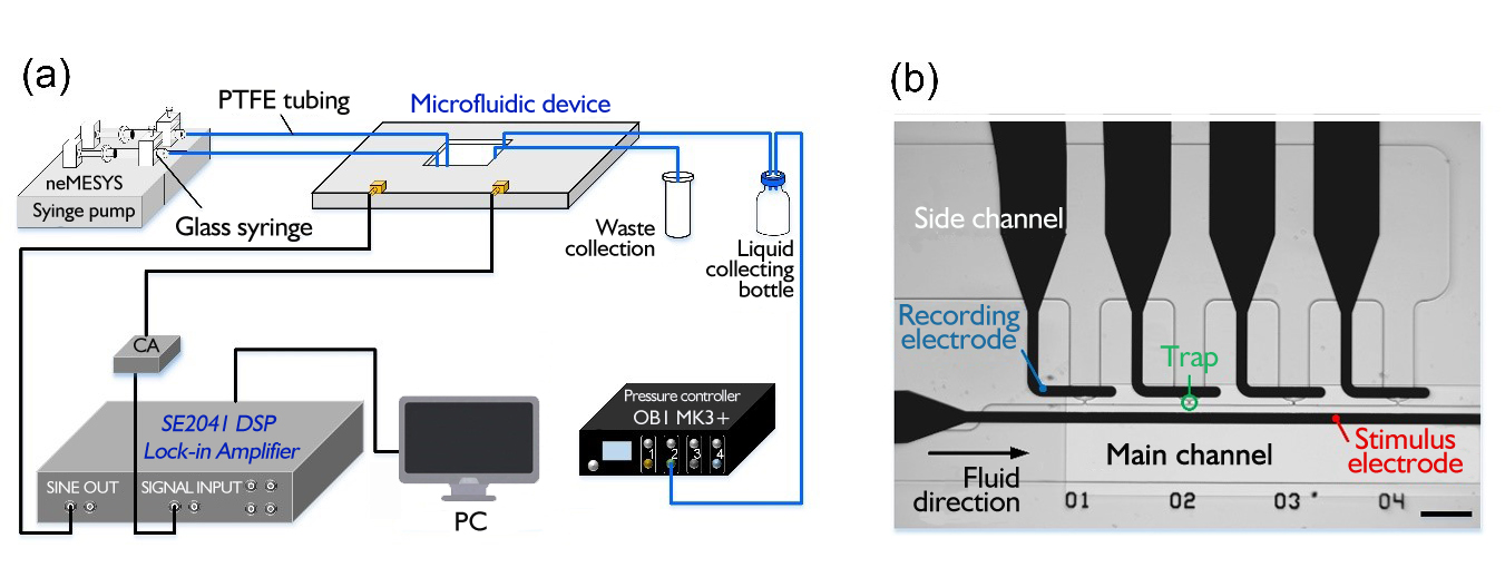
Figure 1 (a). Diagram of the microfluidic impedance measurement (b). Micrograph of the microfluidic device (scale bar is 100 μm )

As shown in Figure 1, the cell suspension enters the Microfluidic device via a syringe pump through PTFE tubing. The suspension flow rate was maintained at 0.5 µL/min. The pressure provided by the pressure controller makes the inner and outer sides of the trapping hole different in pressure to capture cells or test particles. Then, a digital lock-in amplifier provides a 1Vpp excitation signal to excite the captured cells or test particles, and then measures the current signal fed back into the microfluidic chip. It is converted into a voltage signal by a current amplifier to facilitate the measurement of a digital lock-in amplifier. The data is then collected by a computer and the impedance information of the cells is calculated.

Because the differential current measurement method was used in the experiment to measure the change in current, the background signal from the fluid was largely suppressed. This makes the measured current signal clearer and facilitates inference of cell size and velocity.

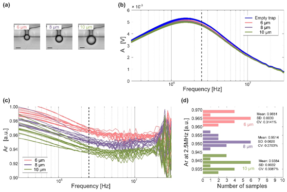
Figure 2  Cell microfluidic impedance measurements (scale bar is 5 µm )

In the amplitude-frequency response curve (Figure 2-b), the amplitude-frequency response curves of no captured particles and captured different particles are mixed in the low-frequency domain and high-frequency domain, and it is difficult to distinguish. And it is also hard to determine the amplitude-frequency response curve alone. The best frequency point is used to distinguish particles, so the measured amplitude-frequency response curve is normalized, that is, the calculation is performed as shown in the following formula.

Ar = A * Ae

After normalization, it can be seen that the amplitudes measured at 2.5 MHz are the easiest to distinguish between the different particles. Therefore, after fixing the frequency of the input excitation signal to 2.5 MHz, we re-measure different particles several times and obtain results shown in Figure 2-d.

Based on the results, we can see the results obtained after multiple sets of measurements for different particles: 6 µm particles have an average amplitude of 0.9651, a standard deviation (SD) of 0.0030, and a volatility coefficient (CV) of 0.3141%; 8 µm particles have an average amplitude of 0.9651 0.9514, the standard deviation is 0.0028, and the fluctuation coefficient is 0.2703%; the average amplitude of 10 µm particles is 0.9384, the standard deviation is 0.0032, and the fluctuation coefficient is 0.3387%. The extremely small standard deviation and fluctuation coefficient show that the sensitivity and stability of this measurement are very high, and the significantly different amplitude averages are also strong evidence for distinguishing particles.

Therefore, using a digital lock-in amplifier to construct a microfluidic device for electrical impedance spectroscopy measurement is currently the most effective way.